3 LandR Biomass_borealDataPrep Module

3.0.0.1 Authors:

Yong Luo yong.luo@canada.ca [aut], Eliot J B McIntire eliot.mcintire@nrcan-rncan.gc.ca [aut, cre], Ceres Barros ceres.barros@ubc.ca [aut], Alex M. Chubaty achubaty@for-cast.ca [aut]

This documentation is a work in progress. Potential discrepancies and omissions may exist for the time being. If you find any, contact us using the “Get help” link above.

3.1 Module Overview

3.1.1 Quick links

• General functioning

• List of input objects

• List of parameters

• List of outputs

• Simulation flow and module events

3.1.2 Summary

LandR Biomass_borealDataPrep (hereafter Biomass_borealDataPrep), prepares all necessary inputs for Biomass_core based on data available for forests across Canada forests, but focused on Western Canada boreal forest systems. Nevertheless, it provides a good foundation to develop other modules aimed at different geographical contexts. By keeping data preparation and parameter estimation outside of Biomass_core, we promote the modularity of the LandR-based model systems and facilitate interoperability with other parameter estimation procedures.

Specifically, it prepares and adjusts invariant and spatially-varying species trait values, as well as ecolocation-specific parameters, probabilities of germination and initial conditions necessary to run Biomass_core. For this, Biomass_borealDataPrep requires internet access to retrieve default data⁸.

We advise future users to run Biomass_borealDataPrep with defaults and inspect the resulting input objects are like before supplying alternative data (or data URLs).

3.1.3 Links to other modules

Biomass_borealDataPrep is intended to be used with Biomass_core, but can be linked with other data modules that prepare inputs. See here for all available modules in the LandR ecosystem and select Biomass_borealDataPrep from the drop-down menu to see potential linkages.

• Biomass_core: core forest dynamics simulation module. Used downstream from Biomass_borealDataPrep;

• Biomass_speciesData: grabs and merges several sources of species cover data, making species percent cover (% cover) layers used by other LandR Biomass modules. Default source data spans the entire Canadian territory. Used upstream from Biomass_borealDataPrep;

• Biomass_speciesParameters: calibrates four-species level traits using permanent sample plot data (i.e., repeated tree biomass measurements) across Western Canada. Used downstream from Biomass_borealDataPrep.

3.2 Module manual

3.2.1 General functioning

Biomass_borealDataPrep prepares all inputs necessary to run a realistic simulation of forest dynamics in Western Canadian boreal forests using Biomass_core. Part of this process involves cleaning up the input data and imputing missing data in some cases, which are discussed in detail in Data acquisition and treatment.

After cleaning and formatting the raw input data, the module:

1. calculates species biomass per pixel by multiplying the observed species % cover by the observed stand biomass and an adjustment factor, which can be statistically calibrated for the study area. Given that this adjusts the species biomass, this calibration step contributes to the calibration of maxB and maxANPP trait values, whose estimation is also based on species biomass (see Initial species age and biomass per pixel and Adjustment of species biomass);

2. prepares invariant species traits – these are spatio-temporally constant species traits that influence population dynamics (e.g., growth, mortality, dispersal) and responses to fire (see Invariant species traits);

3. defines ecolocations – groupings of pixels with similar biophysical conditions. By default, ecolocations are defined as the spatial combination of ecodistricts of the National Ecological Framework for Canada, and the Land Cover of Canada 2010 map (see Defining simulation pixels and ecolocations). Note that ecolocation is termed ecoregionGroup across LandR modules.

4. prepares ecolocation-specific parameters and probabilities of germination – only one ecolocation-specific parameter is used, the minimum relative biomass thresholds, which defines the level of shade in a pixel. Together the level of shade and the probabilities of germination influence germination success in any given pixel;

5. estimates spatio-temporally varying species traits – species traits that can vary by ecolocation and in time. These are maximum biomass (maxB), maximum above-ground net primary productivity (maxANPP; see Maximum biomass and maximum aboveground net primary productivity) and species establishment probability (SEP, called establishprob in the module traits table; see Species establishment probability). By default, Biomass_borealDataPrep estimates temporally constant values of maxB, maxANPP and SEP;

6. creates initial landscape conditions – Biomass_borealDataPrep performs data-based landscape initialisation, by creating the species cohort table (cohortData) and corresponding map (pixelGroupMap; both used to initialise and track cohorts across the landscape) based on observed stand age and species biomass.

As Biomass_core only simulates tree species dynamics, Biomass_borealDataPrep prepares all inputs and estimates parameters in pixels within forested land-cover classes (see Defining simulation pixels and ecolocations).

If a studyAreaLarge is supplied, the module uses it for parameter estimation to account for larger spatial variability.

In the next sections, we describe in greater detail the various data processing and parameter estimation steps carried out by Biomass_borealDataPrep.

3.2.2 Data acquisition and treatment

The only two objects that the user must supply are shapefiles that define the study area used to derive parameters (studyAreaLarge) and the study area where the simulation will happen (studyArea). The two objects can be identical if the user chooses to parametrise and run the simulations in the same area. If not identical, studyArea must be fully within studyAreaLarge. If studyAreaLarge and studyArea are in Canada, the module can automatically estimate and prepare all input parameters and objects for Biomass_core, as the default raw data are FAIR data (sensu Wilkinson et al. 2016) at the national-scale.

If no other inputs are supplied, Biomass_borealDataPrep will create raster layer versions studyAreaLarge and studyArea (rasterToMatchLarge and rasterToMatch, respectively), using the stand biomass map layer (rawBiomassMap) as a template (i.e., the source of information for spatial resolution).

3.2.2.1 Defining simulation pixels and ecolocations

Biomass_borealDataPrep uses land-cover data to define and assign parameter values to the pixels where forest dynamics will be simulated (forested pixels). By default it uses land-cover classes from the Land Cover of Canada 2010 v1 map, a raster-based database that distinguishes several forest and non-forest land-cover types. Pixels with classes 1 to 6 are included as forested pixels (see parameter forestedLCCClasses).

When the land-cover raster (rstLCC) includes transient cover types (e.g., recent burns) the user may pass a vector of transient class IDs (via the parameter LCCClassesToReplaceNN) that will be reclassified into a “stable” forested class (defined via the parameter forestedLCCClasses). The reclassification is done by searching the focal neighbourhood for a replacement forested cover class (up to a radius of 1250m from the focal cell). If no forested class is found within this perimeter, the pixel is not used to simulate forest dynamics. Reclassified pixels are omitted from the fitting of statistical models used for parameter estimation, but are assigned predicted values from these models.

Sub-regional spatial variation in maxBiomass, maxANPP, and SEP species traits is accounted for by ecolocation. Ecolocations are used as proxies for biophysical variation across the landscape when estimating model parameters that vary spatially. By default, they are defined as the combination of “ecodistricts” from the National Ecological Framework for Canada (a broad-scale polygon layer that captures sub-regional variation) (ecoregionLayer) and the above land cover (rstLCC), but the user can change this by supplying different ecozonation or land-cover layers.

3.2.2.2 Species cover

Species cover (% cover) raster layers (speciesLayers) can be automatically obtained and pre-processed by Biomass_borealDataPrep. The module ensures that:

1. all data have the same geospatial properties (extent, resolution);
2. all layers these are correctly re-projected to studyAreaLarge and rasterToMatchLarge;
3. species with no cover values above 10% are excluded.

By default it uses species % cover rasters derived from the MODIS satellite imagery from 2001, obtained from the Canadian National Forest Inventory (Beaudoin et al. 2017) – hereafter ‘kNN species data’.

3.2.2.3 Initial species age and biomass per pixel

Stand age and aboveground stand biomass (hereafter ‘stand biomass’) are used to derive parameters and define initial species age and biomass across the landscape. These are also derived from MODIS satellite imagery from 2001 prepared by the NFI (Beaudoin et al. 2017) by default.

Biomass_borealDataPrep downloads these data and performs a number of data harmonization operations to deal with data inconsistencies. It first searches for mismatches between stand age (standAge), stand biomass (standB) and total stand cover (standCover), assuming that cover is the most accurate of the three, and biomass the least, and in the following order:

1. Pixels with standCover < 5% are removed;

2. Pixels with standAge == 0, are assigned standB == 0;

3. Pixels with standB == 0, are assigned standAge == 0.

Then, species is assigned one cohort per pixel according to the corrected stand age, stand biomass and % cover values. Cohort age is assumed to be the same as stand age and biomass is the product of stand biomass and species % cover. Before doing so, stand cover is rescaled to vary between 0 and 100%.

A next set of data inconsistencies in cohort age (age), biomass (B) and cover (cover) is looked for and solved in the following order:

4. if cover > 0 and age == 0, B is set to 0 (and stand biomass recalculated);

5. if cover == 0 and age > 0, or if age == NA, age is empirically estimated using the remainder of the data to fit the model supplied by P(sim)$imputeBadAgeModel, which defaults to:

## [[1]]
## lme4::lmer(age ~ log(totalBiomass) * cover * speciesCode + (log(totalBiomass) | 
##     initialEcoregionCode))

Cohort biomass is then adjusted to reflect the different cover to biomass relationship of conifer and broadleaf species (see Adjustment of initial species biomass).

Finally, Biomass_borealDataPrep can use fire perimeters to correct stand ages. To do so, it downloads the latest fire perimeter data from the Canadian Wildfire Data Base and changes pixel age inside fire perimeters to match the time since last fire, using fire years up to the first year of the simulation.

This assumes that the 1) last fire was a stand replacing fire and 2) that the first year of the simulation is later than the first fire year in the fire perimeter data. If the user does not want to assume 1), this data imputation step can be bypassed by setting the parameter P(sim)$overrideBiomassInFires to FALSE or P(sim)$fireURL to NULL or NA.

In pixels where ages are changed to match time since the last fire, cohort biomass needs to be corrected – in our default datasets we have noticed biomass is inflated in pixels with recent burns. Consequently, the module uses a spin-up simulation that grows cohorts to their fixed age inside each pixel using estimated maxB and maxANPP parameters (see Maximum biomass and maximum aboveground net primary productivity).

Note that pixels that had data imputation can be removed from the simulation by setting P(sim)$rmImputedPix == TRUE.

3.2.2.4 Invariant species traits

Most invariant species traits are obtained from available species trait tables used in LANDIS-II applications in Canada’s boreal forests (available in Dominic Cyr’s GitHub repository). Some are then adapted with minor adjustments to match Western Canadian boreal forests using published literature. Others (key growth and mortality traits) can be calibrated by Biomass_speciesParameters (see Calibrating species growth/mortality traits using Biomass_speciesParameters).

The LANDIS-II species trait table contains species trait values for each Canadian Ecozone (NRCan 2013), which are by default filtered to the Boreal Shield West (BSW), Boreal Plains (BP) and Montane Cordillera Canadian Ecozones (via P(sim)$speciesTableAreas). Most trait values do not vary across these ecozones for a given species, but when they do the minimum value is used.

The function LandR::speciesTableUpdate is used by default to do further adjustments to trait values in this table (if this is not intended, a custom function call or NULL can be passed to P(sim)$speciesUpdateFunction):

• Longevity values are adjusted to match the values from Burton & Cumming (1995b), which match BSP, BP and MC ecozones. These adjustments result in higher longevity for most species;

• Shade tolerance values are lowered for Abies balsamifera, Abies lasiocarpa, Picea engelmanii, Picea glauca, Picea mariana, Tsuga heterophylla and Tsuga mertensiana to better relative shade tolerance levels in Western Canada. Because these are relative shade tolerances, the user should always check these values with respect to their own study areas and species pool.

The user can also pass more than one function call to P(sim)$speciesUpdateFunction if they want to make other adjustments in addition to those listed above (see ?LandR::updateSpeciesTable).

3.2.2.5 Probabilities of germination

By default, Biomass_borealDataPrep uses the same probabilities of germination (called sufficientLight in the module) as Biomass_core. These are obtained from publicly available LANDIS-II table.

3.2.3 Parameter estimation/calibration

3.2.3.1 Adjustment of initial species biomass

Biomass_borealDataPrep estimates initial values of species aboveground biomass (B) based on stand biomass (standB) and individual species % cover. Initial B is estimated for each species in each pixel by multiplying standB by species % cover. Because the default cover layers are satellite-derived, the relationship between relative cover and relative biomass of broadleaf and conifer species needs to be adjusted to reflect their different canopy architectures (using P(sim)$deciduousCoverDiscount).

By default, Biomass_borealDataPrep uses a previously estimated P(sim)$deciduousCoverDiscount based on Northwest Territories data. However, the user can chose to re-estimate it by setting P(sim)$fitDeciduousCoverDiscount == TRUE. In this case, by default Biomass_borealDataPrep will fit the the following model:

## [[1]]
## glm(I(log(B/100)) ~ logAge * I(log(totalBiomass/100)) * speciesCode * 
##     lcc)

which relates the estimated biomass (B) with an interaction term between log-age (logAge), standB (‘totalBiomass’), speciesCode (i.e. species ID) and land cover (‘lcc’). The model is fitted to the standB and species cover on studyAreaLarge, using an optimization routine that searches for the best conversion factor between broadleaf species cover and B by minimizing AIC.

3.2.3.2 Maximum biomass and maximum aboveground net primary productivity

Biomass_borealDataPrep statistically estimates maximum biomass (maxB) and maximum aboveground net primary productivity (maxANPP) using the processed species ages and biomass.

maxB is estimated by modelling the response of species biomass (B) to species age and cover, while accounting for variation between ecolocations (ecoregionGroup below):

## [[1]]
## lme4::lmer(B ~ logAge * speciesCode + cover * speciesCode + (logAge + 
##     cover | ecoregionGroup))

The coefficients are estimated by maximum likelihood and model fit is calculated as the proportion of explained variance explained by fixed effects only (marginal r2) and by the entire model (conditional r2) – both of which are printed as messages.

Because the model can take a while to fit, by default we sample pixels within each species and ecolocation combination (sample size defined by the P(sim)$subsetDataBiomassModel parameter).

If convergence issues occur and P(sim)$fixModelBiomass == TRUE, the module attempts to refit the model by re-sampling the data, re-fitting lmer with the bobyqa optimizer, and re-scaling the continuous predictors (by default, cover and logAge). These steps are tried additively until the convergence issue is resolved. If the module is still unable to solve the convergence issue a message is printed and the module uses the last fitted model.

Note that convergence issues are not usually problematic for the estimation of coefficient values, only for estimation of their standard errors. However, the user should always inspect the final model (especially if not converged) and make sure that the problems are not significant and that the fitted model meets residual assumptions. For this, the user should make sure model objects are exported to the simList using the exportModels parameter.

Alternative model calls/formulas can be supplied via the P(sim)$biomassModel parameter. Note that if supplying a model call that does not use lme4::lmer the refitting process is likely to fail and may have to be disabled (via the P(sim)$fixModelBiomass parameter).

Another consideration to add with respect to the estimation of maxB, is that we are choosing a linear model to relate B ~ log(age) + cover. This is not ideal from an ecological point of view, as biomass is unlikely to vary linearly with age or cover, and more likely to saturate beyond a certain high value of cover and follow a hump-shaped curve with age (i.e., reaching maximum values for a given age, and then starting to decrease as trees approach longevity). Also, fitting a linear model can lead to negative B values at young ages and low cover. However, our tests revealed that a linear mixed effects model was not producing abnormal estimates of B at maximum values of age and cover (hence, maxB estimates), while allowing to leverage on the powerful statistical machinery of lme4.

Finally, we highlight that modelling log(B) is NOT an appropriate solution, because it will wrongly assume an exponential relationship between B ~ log(age) + cover, leading to a serious overestimation of maxB(Fig. 3.1) and steep increases in species biomasses during the first years of the simulation (Fig. 3.2).

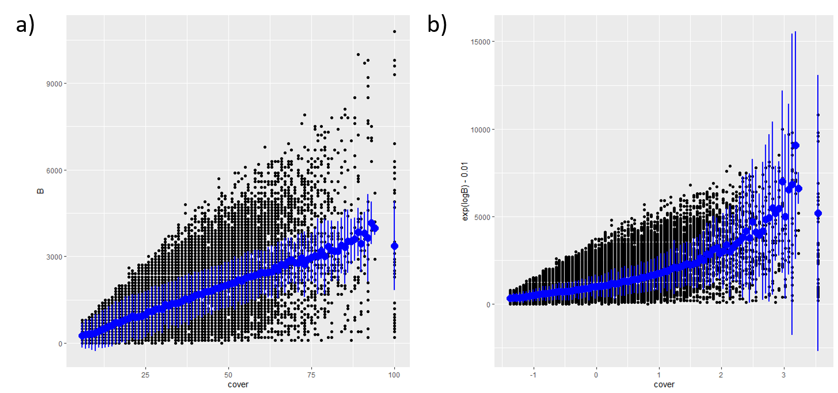
Figure 3.1: Modelling biomass as a linear vs. exponential relationship. a) modelBiomass as B ~ logAge * speciesCode + cover * speciesCode + (logAge + cover | ecoregionGroup). b) modelBiomass as logB ~ logAge * speciesCode + cover * speciesCode + (logAge + cover | ecoregionGroup). Blue dots are marginal mean B values (back-transformed in b) cross ages with confidence intervals as the bars.

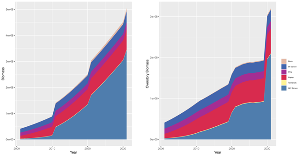
Figure 3.2: Thirty years of simulation with maxB values estimated from a logB ~ ... biomassModel (see Fig. 3.1). The steep increase in such little time is abnormal.

After the biomass model is fit, maxB is predicted by species and ecolocation combination, for maximum species cover values (100%) and maximum log-age (the log of species longevity). When using Biomass_speciesParameters, maxB is calibrated so that species can achieve the maximum observed biomass during the simulation (see Calibrating species growth/mortality traits using Biomass_speciesParameters).

maxANPP is the calculated as maxB * mANPPproportion/100, where mANPPproportion defaults to 3.33, unless calibrated by Biomass_speciesParameters (see Calibrating species growth/mortality traits using Biomass_speciesParameters). The default value, 3.33, comes from an inversion of the rationale used to calculate maxB in Scheller & Mladenoff (2004). There, the authors estimated maxANPP using the model PnET-II (and then adjusted the values manually) and from these estimates calculated maxB by multiplying the estimated maxANPP by 30.

3.2.3.3 Species establishment probability

Species establishment probability (SEP, establishprob in the module) is estimated by modelling the probability of observing a given species in each ecolocation. For this, Biomass_borealDataPrep models the relationship between probability of occurrence of a species (\(\pi\)) using the following model by default:

## [[1]]
## glm(cbind(coverPres, coverNum - coverPres) ~ speciesCode * ecoregionGroup, 
##     family = binomial)

whereby the probability of occurrence of a species (\(\pi\)) – calculated as the proportion of pixels with % cover > 0 – is modelled per species and ecolocation following a binomial distribution with a logit link function. There is no data sub-sampling done before fitting the SEP statistical model, as the model fits quickly even for very large sample sizes (e.g., > 20 million points).

SEP is then predicted by species and ecolocation combination and the resulting values are integrated over the length of the succession time step (successionTimestep parameter) as:

\[\begin{equation} integratedSEP = 1-(1-estimatedSEP)^{e^{successionTimestep}} \tag{3.1} \end{equation}\]

This is important, since seed establishment only occurs once at every P(sim)$successionTimestep, and thus the probabilities of seed establishment need to be temporally integrated to reflect the probability of a seed establishing in this period of time.

Finally, since the observed species cover used to fit coverModel is a result of both seed establishment and resprouting/clonal growth, the final species establishment probabilities are calculated as a function of the temporally integrated presence probabilities and species’ probabilities of resprouting (resproutprob, in the species table) (bounded between 0 and 1):

\[\begin{equation} SEP = integratedSEP * (1 - resproutprob) \tag{3.2} \end{equation}\]

if \(SEP > 1\), then:

\[\begin{equation} SEP = 1 \tag{3.3} \end{equation}\]

if \(SEP < 0\), then:

\[\begin{equation} SEP = 0 \tag{3.4} \end{equation}\]

3.2.3.4 Ecolocation-specific parameter – minimum relative biomass

Minimum relative biomass (minRelativeB) is a spatially-varying parameter used to determine the shade level in each pixel. Each shade class (X0-X5) is defined by a minimum relative biomass threshold compared to the pixel’s current relative biomass, which is calculated as the sum of pixel’s total biomass divided by the total potential maximum biomass in that pixel (the sum of all maxB for the pixel’s ecolocation).

Since we found no data to base the parametrisation of the shade class thresholds, default values are based on publicly available values used in LANDIS-II applications in Canada’s boreal forests (available in Dominic Cyr’s GitHub repository), and all ecolocations share the same values.

Initial runs revealed excessive recruitment of moderately shade-intolerant species even as stand biomass increased, so values for shade levels X4 and X5 are adjusted downwards (X4: 0.8 to 0.75; X5: 0.90 to 0.85) to reflect higher competition for resources (e.g. higher water limitation) in Western Canadian forests with regards to Eastern Canadian forests (Messier et al. 1998), which are likely driven by higher moisture limitation in the west (Hogg et al. 2008; Peng et al. 2011).

This adjustment can be bypassed by either supplying a minRelativeB table, or an alternative function call to P(sim)$minRelativeBFunction (which by default is LandR::makeMinRelativeB.

The minimum biomass threshold of a shade level of X0 is 0 standB.

3.2.3.5 Calibrating species growth/mortality traits using Biomass_speciesParameters

If using Biomass_borealDataPrep and Biomass_speciesParameters, the later module calibrates several species traits that are first prepared by Biomass_borealDataPrep:

• growthcurve, mortalityshape – which initially come from publicly available LANDIS-II tables;

• maxBiomass, maxANPP – which are estimated statistically by Biomass_borealDataPrep (see Maximum biomass and maximum aboveground net primary productivity).

Briefly, Biomass_speciesParameters:

1. Uses ~41,000,000 hypothetical species’ growth curves (generated with Biomass_core), that cover a fully factorial combination of longevity, ratio of maxANPP to maxBiomass, growthcurve, mortalityshape;

2. Takes permanent and temporary sample plot (PSP) data in or near the study area for the target species, and finds which hypothetical species’ growth curve most closely matches the growth curve observed in the PSP data – on a species-by-species base. This gives us each species’ growthcurve, mortalityshape, and a new species trait, mANPPproportion, a ratio of maximum aboveground net primary productivity (maxANPP) to maximum biomass (maxBiomass, not to be confounded with maxB) in the study area.

3. Introduces a second new species trait, inflationFactor, and re-calibrates maxB. We recognize that maxB, as obtained empirically by Biomass_borealDataPrep, cannot be easily reached in simulations because all reasonable values of growthcurve, mortalityshape and longevity prevent the equation from reaching maxB (it acts as an asymptote that is never approached). The inflationFactor is calculated as the ratio of maxBiomass (the parameter used to generate theoretical growth curves in step 1) to the maximum biomass actually achieved by the theoretical growth curves (step 1). maxB is then recalibrated by multiplying it by inflationFactor. By doing this, resulting non-linear growth curves generated doing Biomass_core simulation will be able to achieve the the empirically estimated maxB.

4. Estimates species-specific maxANPP by multiplying the final maxB above by mANPPproportion (estimated in step 2).

In cases where there is insufficient PSP data to perform the above steps, maxB and maxANPP are left as estimated by Biomass_borealDataPrep (see Maximum biomass and maximum aboveground net primary productivity) and inflationFactor and mANPPproportion take default values of 1 and 3.33.

3.2.4 Aggregating species

Biomass_borealDataPrep will use the input table sppEquiv and the parameter P(sim)$sppEquivCol to select the naming convention to use for the simulation (see full list of input objects and parameters for details). The user can use this table and parameter to define groupings that “merge” similar species that have their own invariant trait values (see Invariant species traits) (e.g. genus-level group or a functional group). To do so, the name of the species group in sppEquivCol column of the sppEquiv table must be identical for each grouped species.

Table 3.1: Example of species merging for simulation. Here the user wants to model Abies balsamea, A. lasiocarpa and Pinus contorta as separate species, but all Picea spp. as a genus-level group. For this, all six species are identified in the ‘KNN’ column, so that their % cover layers can be obtained, but in the ‘Boreal’ column (which defines the naming convention used in the simulation in this example) all Picea spp. have the same name. Biomass_borealDataPrep will merge their % cover data into a single layer by summing their cover per pixel.

Species	KNN	Boreal	Modelled as
Abies balsamea	Abie_Bal	Abie_Bal	Abies balsamea
Abies lasiocarpa	Abie_Las	Abie_Las	Abies lasiocarpa
Picea engelmannii x glauca	Pice_Eng_Gla	Pice_Spp	Picea spp.
Picea engelmannii x glauca	Pice_Eng_Gla	Pice_Spp	Picea spp.
Picea engelmannii	Pice_Eng	Pice_Spp	Picea spp.
Picea glauca	Pice_Gla	Pice_Spp	Picea spp.
Picea mariana	Pice_Mar	Pice_Spp	Picea spp.
Pinus contorta var. contorta		Pinu_Con	Pinus contorta var. contorta
Pinus contorta	Pinu_Con	Pinu_Con	Pinus contorta

When groups contain species with different (invariant) trait values, the minimum value across all species is used. As for the default species % cover layers, Biomass_borealDataPrep proceeds in the same way as Biomass_speciesData and sums cover across species of the same group per pixel.

3.2.5 List of input objects

Below are is the full lists of input objects (Table 3.2) that Biomass_borealDataPrep expects.

The only inputs that must be provided (i.e., Biomass_borealDataPrep does not have a default for) are studyArea (the study area used to simulate forest dynamics Biomass_core) and studyAreaLarge (a potentially larger study area used to derive parameter values – e.g., species traits).

All other input objects and parameters have internal defaults.

Of these inputs, the following are particularly important and deserve special attention:

Spatial layers

• ecoregionLayer or ecoregionRst – a shapefile or map containing ecological zones.

• rawBiomassMap – a map of observed stand biomass (in \(g/m^2\)).

• rstLCC – a land-cover raster.

• speciesLayers – layers of species % cover data. The species must match those available in default (or provided) species traits tables (the species and speciesEcoregion tables).

• standAgeMap – a map of observed stand ages (in years).

• studyArea – shapefile. A SpatialPolygonsDataFrame with a single polygon determining where the simulation will take place. This input object must be supplied by the user.

• studyAreaLarge – shapefile. A SpatialPolygonsDataFrame with a single polygon determining the where the statistical models for parameter estimation will be fitted. It must contain studyArea fully, if they are not identical. This object must be supplied by the user.

Tables

• speciesTable – a table of invariant species traits that must have the following columns (even if not all are necessary to the simulation): “species”, “Area”, “longevity”, “sexualmature”, “shadetolerance”, “firetolerance”, “seeddistance_eff”, “seeddistance_max”, “resproutprob”, “resproutage_min”, “resproutage_max”, “postfireregen”, “leaflongevity”, “wooddecayrate”, “mortalityshape”, “growthcurve”, “leafLignin”, “hardsoft”. The order can vary but the column names must be identical. See Scheller & Miranda (2015a) and Biomass_core manual for further detail about these columns.

Table 3.2: List of Biomass_borealDataPrep input objects and their description.

objectName	objectClass	desc	sourceURL
cloudFolderID	character	The google drive location where cloudCache will store large statistical objects	NA
columnsForPixelGroups	character	The names of the columns in cohortData that define unique pixelGroups. Default is c(‘ecoregionGroup’, ‘speciesCode’, ‘age’, ‘B’)	NA
ecoregionLayer	SpatialPolygonsDataFrame	A SpatialPolygonsDataFrame that characterizes the unique ecological regions (ecoregionGroup) used to parameterize the biomass, cover, and species establishment probability models. It will be overlaid with landcover to generate classes for every ecoregion/LCC combination. It must have same extent and crs as studyAreaLarge. It is superseded by sim$ecoregionRst if that object is supplied by the user	https://sis.agr.gc.ca/cansis/nsdb/ecostrat/district/ecodistrict_shp.zip
ecoregionRst	RasterLayer	A raster that characterizes the unique ecological regions used to parameterize the biomass, cover, and species establishment probability models. If this object is provided, it will supercede sim$ecoregionLayer. It will be overlaid with landcover to generate classes for every ecoregion/LCC combination. It must have same extent and crs as rasterToMatchLarge if supplied by user - use reproducible::postProcess. If it uses an attribute table, it must contain the field ‘ecoregion’ to represent raster values	NA
rstLCC	RasterLayer	A land classification map in study area. It must be ‘corrected’, in the sense that: 1) Every class must not conflict with any other map in this module (e.g., speciesLayers should not have data in LCC classes that are non-treed); 2) It can have treed and non-treed classes. The non-treed will be removed within this module if P(sim)$omitNonTreedPixels is TRUE; 3) It can have transient pixels, such as ‘young fire’. These will be converted to a the nearest non-transient class, probabilistically if there is more than 1 nearest neighbour class, based on P(sim)$LCCClassesToReplaceNN. The default layer used, if not supplied, is Canada national land classification in 2010. The metadata (res, proj, ext, origin) need to match rasterToMatchLarge.	NA
rasterToMatch	RasterLayer	A raster of the studyArea in the same resolution and projection as rawBiomassMap. This is the scale used for all outputs for use in the simulation. If not supplied will be forced to match the default rawBiomassMap.	NA
rasterToMatchLarge	RasterLayer	A raster of the studyAreaLarge in the same resolution and projection as rawBiomassMap. This is the scale used for all inputs for use in the simulation. If not supplied will be forced to match the default rawBiomassMap.	NA
rawBiomassMap	RasterLayer	total biomass raster layer in study area. Defaults to the Canadian Forestry Service, National Forest Inventory, kNN-derived total aboveground biomass map from 2001 (in tonnes/ha), unless ‘dataYear’ != 2001. If necessary, biomass values are rescaled to match changes in resolution. See https://open.canada.ca/data/en/dataset/ec9e2659-1c29-4ddb-87a2-6aced147a990 for metadata.	http://ftp.maps.canada.ca/pub/nrcan_rncan/Forests_Foret/canada-forests-attributes_attributs-forests-canada/2001-attributes_attributs-2001/NFI_MODIS250m_2001_kNN_Structure_Biomass_TotalLiveAboveGround_v1.tif
speciesLayers	RasterStack	cover percentage raster layers by species in Canada species map. Defaults to the Canadian Forestry Service, National Forest Inventory, kNN-derived species cover maps from 2001 using a cover threshold of 10 - see https://open.canada.ca/data/en/dataset/ec9e2659-1c29-4ddb-87a2-6aced147a990 for metadata	http://ftp.maps.canada.ca/pub/nrcan_rncan/Forests_Foret/canada-forests-attributes_attributs-forests-canada/2001-attributes_attributs-2001/
speciesTable	data.table	a table of invariant species traits with the following trait colums: ‘species’, ‘Area’, ‘longevity’, ‘sexualmature’, ‘shadetolerance’, ‘firetolerance’, ‘seeddistance_eff’, ‘seeddistance_max’, ‘resproutprob’, ‘resproutage_min’, ‘resproutage_max’, ‘postfireregen’, ‘leaflongevity’, ‘wooddecayrate’, ‘mortalityshape’, ‘growthcurve’, ‘leafLignin’, ‘hardsoft’. Names can differ, but not the column order. Default is from Dominic Cyr and Yan Boulanger’s project	https://raw.githubusercontent.com/dcyr/LANDIS-II_IA_generalUseFiles/master/speciesTraits.csv
sppColorVect	character	named character vector of hex colour codes corresponding to each species	NA
sppEquiv	data.table	table of species equivalencies. See ?LandR::sppEquivalencies_CA.	NA
sppNameVector	character	an optional vector of species names to be pulled from sppEquiv. If not provided, then species will be taken from the entire P(sim)$sppEquivCol in sppEquiv. See LandR::sppEquivalencies_CA.	NA
standAgeMap	RasterLayer	stand age map in study area. Defaults to the Canadian Forestry Service, National Forest Inventory, kNN-derived biomass map from 2001, unless ‘dataYear’ != 2001. See https://open.canada.ca/data/en/dataset/ec9e2659-1c29-4ddb-87a2-6aced147a990 for metadata	http://ftp.maps.canada.ca/pub/nrcan_rncan/Forests_Foret/canada-forests-attributes_attributs-forests-canada/2001-attributes_attributs-2001/NFI_MODIS250m_2001_kNN_Structure_Stand_Age_v1.tif
studyArea	SpatialPolygonsDataFrame	Polygon to use as the study area. Must be supplied by the user.	NA
studyAreaLarge	SpatialPolygonsDataFrame	multipolygon (potentially larger than studyArea) used for parameter estimation, Must be supplied by the user. If larger than studyArea, it must fully contain it.	NA

3.2.6 List of parameters

Table 3.3 lists all parameters used in Biomass_borealDataPrep and their detailed information. All have default values specified in the module’s metadata.

Of these parameters, the following are particularly important:

Estimation of simulation parameters

• biomassModel – the statistical model (as a function call) used to estimate maxB and maxANPP.

• coverModel – the statistical model (as a function call) used to estimate SEP.

• fixModelBiomass – determines whether biomassModel is re-fit when convergence issues arise.

• imputeBadAgeModel – model used to impute ages when they are missing, or do not match the input cover and biomass data. Not to be confounded with correcting ages from fire data

• subsetDataAgeModel and subsetDataBiomassModel – control data sub-sampling for fitting the imputeBadAgeModel and biomassModel, respectively

• exportModels – controls whether biomassModel or coverModel (or both) are to be exported in the simulation simList, which can be useful to inspect the fitted models and report on statistical fit.

• sppEquivCol – character. the column name in the speciesEquivalency data.table that defines the naming convention to use throughout the simulation.

Data processing

• forestedLCCClasses and LCCClassesToReplaceNN – define which land-cover classes in rstLCC are forested and which should be reclassified to forested classes, respectively.

• deciduousCoverDiscount, coverPctToBiomassPctModel and fitDeciduousCoverDiscount – the first is the adjustment factor for broadleaf species cover to biomass relationships; the second and third are the model used to refit deciduousCoverDiscount in the supplied studyAreaLarge and whether refitting should be attempted (respectively).

Table 3.3: List of Biomass_borealDataPrep parameters and their description.

paramName	paramClass	default	min	max	paramDesc
biomassModel	call	lme4::lm….	NA	NA	Model and formula for estimating biomass (B) from ecoregionGroup (currently ecoregionLayer LandCoverClass), speciesCode, logAge (gives a downward curving relationship), and cover. Defaults to a LMEM, which can be slow if dealing with very large datasets (e.g. 36 000 points take 20min). For faster fitting try P(sim)$subsetDataBiomassModel == TRUE, or quote(RcppArmadillo::fastLm(formula = B ~ logAge speciesCode ecoregionGroup + cover speciesCode ecoregionGroup)). A custom model call can also be provided, as long as the ‘data’ argument is NOT included.
coverModel	call	glm, cbi….	NA	NA	Model and formula used for estimating cover from ecoregionGroup and speciesCode and potentially others. Defaults to a GLMEM if there are > 1 grouping levels. A custom model call can also be provided, as long as the ‘data’ argument is NOT included
coverPctToBiomassPctModel	call	glm, I(l….	NA	NA	Model to estimate the relationship between % cover and % biomass, referred to as P(sim)$fitDeciduousCoverDiscount It is a number between 0 and 1 that translates % cover, as provided in several databases, to % biomass. It is assumed that all hardwoods are equivalent and all softwoods are equivalent and that % cover of hardwoods will be an overesimate of the % biomass of hardwoods. E.g., 30% cover of hardwoods might translate to 20% biomass of hardwoods. The reason this discount exists is because hardwoods in Canada have a much wider canopy than softwoods.
deciduousCoverDiscount	numeric	0.8418911	NA	NA	This was estimated with data from NWT on March 18, 2020 and may or may not be universal. Will not be used if P(sim)$fitDeciduousCoverDiscount == TRUE
fitDeciduousCoverDiscount	logical	FALSE	NA	NA	If TRUE, this will re-estimate P(sim)$fitDeciduousCoverDiscount This may be unstable and is not recommended currently. If FALSE, will use the current default
dataYear	numeric	2001	NA	NA	Used to override the default ‘sourceURL’ of KNN datasets (species cover, stand biomass and stand age), which point to 2001 data, to fetch KNN data for another year. Currently, the only other possible year is 2011.
ecoregionLayerField	character		NA	NA	the name of the field used to distinguish ecoregions, if supplying a polygon. Defaults to NULL and tries to use ‘ECODISTRIC’ where available (for legacy reasons), or the row numbers of sim$ecoregionLayer. If this field is not numeric, it will be coerced to numeric.
exportModels	character	none	NA	NA	Controls whether models used to estimate maximum B/ANPP (biomassModel) and species establishment (coverModel) probabilities are exported for posterior analyses or not. This may be important when models fail to converge or hit singularity (but can still be used to make predictions) and the user wants to investigate them further. Can be set to ‘none’ (no models are exported), ‘all’ (both are exported), ‘biomassModel’ or ‘coverModel’. BEWARE: because this is intended for posterior model inspection, the models will be exported with data, which may mean very large simList(s)!
fireURL	character	https://….	NA	NA	A URL to a fire database, such as the Canadian National Fire Database, that is a zipped shapefile with fire polygons, an attribute (i.e., a column) named ‘Year’. If supplied (omitted with NULL or NA), this will be used to ‘update’ age pixels on standAgeMap with ‘time since fire’ as derived from this fire polygons map. Biomass is also updated in these pixels, when the last fire is more recent than 1986. If NULL or NA, no age and biomass imputation will be done in these pixels.
fixModelBiomass	logical	FALSE	NA	NA	should modelBiomass be fixed in the case of non-convergence? Only scaling of variables and attempting to fit with a new optimizer are implemented at this time
forestedLCCClasses	numeric	1, 2, 3,….	0	NA	The classes in the rstLCC layer that are ‘treed’ and will therefore be run in Biomass_core. Defaults to forested classes in LCC2010 map.
imputeBadAgeModel	call	lme4::lm….	NA	NA	Model and formula used for imputing ages that are either missing or do not match well with biomass or cover. Specifically, if biomass or cover is 0, but age is not, or if age is missing (NA), then age will be imputed.
LCCClassesToReplaceNN	numeric		NA	NA	This will replace these classes on the landscape with the closest forest class P(sim)$forestedLCCClasses. If the user is using the LCC 2005 land-cover data product for rstLCC, then they may wish to include 36 (cities – if running a historic range of variation project), and 34:35 (burns) Since this is about estimating parameters for growth, it doesn’t make any sense to have unique estimates for transient classes in most cases. If no classes are to be replaced, pass 'LCCClassesToReplaceNN' = numeric(0) when supplying parameters.
minCoverThreshold	numeric	5	0	100	Pixels with total cover that is equal to or below this number will be omitted from the dataset
minRelativeBFunction	call	LandR::m….	NA	NA	A quoted function that makes the table of min. relative B determining a stand shade level for each ecoregionGroup. Using the internal object pixelCohortData is advisable to access/use the list of ecoregionGroups per pixel. The function must output a data.frame with 6 columns, named ecoregionGroup and ‘X1’ to ‘X5’, with one line per ecoregionGroup code, and the min. relative biomass for each stand shade level X1-5. The default function uses values from LANDIS-II available at: https://github.com/dcyr/LANDIS-II_IA_generalUseFiles/blob/master/LandisInputs/BSW/biomass-succession-main-inputs_BSW_Baseline.txt%7E.
omitNonTreedPixels	logical	TRUE	FALSE	TRUE	Should this module use only treed pixels, as identified by P(sim)$forestedLCCClasses?
overrideBiomassInFires	logical	TRUE	NA	NA	should B values be re-estimated using Biomass_core for pixels within the fire perimeters obtained from P(sim)$fireURL, based on their time since fire age?
pixelGroupAgeClass	numeric	params(s….	NA	NA	When assigning pixelGroup membership, this defines the resolution of ages that will be considered ‘the same pixelGroup’, e.g., if it is 10, then 6 and 14 will be the same
pixelGroupBiomassClass	numeric	100	NA	NA	When assigning pixelGroup membership, this defines the resolution of biomass that will be considered ‘the same pixelGroup’, e.g., if it is 100, then 5160 and 5240 will be the same
rmImputedPix	logical	FALSE	NA	NA	Should sim$imputedPixID be removed from the simulation?
speciesUpdateFunction	list	LandR::s….	NA	NA	Unnamed list of (one or more) quoted functions that updates species table to customize values. By default, LandR::speciesTableUpdate is used to change longevity and shade tolerance values, using values appropriate to Boreal Shield West (BSW), Boreal Plains (BP) and Montane Cordillera (MC) ecoprovinces (see ?LandR::speciesTableUpdate for details). Set to NULL if default trait values from speciesTable are to be kept instead. The user can supply other or additional functions to change trait values (see LandR::updateSpeciesTable)
sppEquivCol	character	Boreal	NA	NA	The column in sim$speciesEquivalency data.table to use as a naming convention.
speciesTableAreas	character	BSW, BP, MC	NA	NA	One or more of the Ecoprovince short forms that are in the speciesTable file, e.g., BSW, MC etc. Default is good for Alberta and other places in the western Canadian boreal forests.
subsetDataAgeModel	numeric	50	NA	NA	the number of samples to use when subsampling the age data model and when fitting coverPctToBiomassPctModel; Can be TRUE/FALSE/NULL or numeric; if TRUE, uses 50. If FALSE/NULL no subsetting is done.
subsetDataBiomassModel	numeric		NA	NA	the number of samples to use when subsampling the biomass data model (biomassModel); Can be TRUE/FALSE/NULL or numeric; if TRUE, uses 50. If FALSE/NULL no subsetting is done.
successionTimestep	numeric	10	NA	NA	defines the simulation time step, default is 10 years
useCloudCacheForStats	logical	TRUE	NA	NA	Some of the statistical models take long (at least 30 minutes, likely longer). If this is TRUE, then it will try to get previous cached runs from googledrive.
.plotInitialTime	numeric	start(sim)	NA	NA	This is here for backwards compatibility. Please use .plots
.plots	character	NA	NA	NA	This describes the type of ‘plotting’ to do. See ?Plots for possible types. To omit, set to NA
.plotInterval	numeric	NA	NA	NA	This describes the simulation time interval between plot events
.saveInitialTime	numeric	NA	NA	NA	This describes the simulation time at which the first save event should occur
.saveInterval	numeric	NA	NA	NA	This describes the simulation time interval between save events
.seed	list		NA	NA	Named list of seeds to use for each event (names). E.g., list('init' = 123) will set.seed(123) at the start of the init event and unset it at the end. Defaults to NULL, meaning that no seeds will be set
.sslVerify	integer	64	NA	NA	Passed to httr::config(ssl_verifypeer = P(sim)$.sslVerify) when downloading KNN (NFI) datasets. Set to 0L if necessary to bypass checking the SSL certificate (this may be necessary when NFI’s website SSL certificate is not correctly configured).
.studyAreaName	character	NA	NA	NA	Human-readable name for the study area used. If NA, a hash of studyArea will be used.
.useCache	character	.inputOb….	NA	NA	Internal. Can be names of events or the whole module name; these will be cached by SpaDES

3.2.7 List of outputs

The module produces the following outputs (Table 3.4), which are key inputs of Biomass_core.

Tables

• cohortData – initial community table, containing corrected biomass (g/m2), age and species cover data, as well as ecolocation and pixelGroup information. This table defines the initial community composition and structure used by Biomass_core.

• species – table of invariant species traits. Will contain the same traits as in speciesTable above, but adjusted where necessary.

• speciesEcoregion – table of spatially-varying species traits (maxB, maxANPP, SEP).

• minRelativeB – minimum relative biomass thresholds that determine a shade level in each pixel. X0-5 represent site shade classes from no-shade (0) to maximum shade (5).

• sufficientLight – probability of germination for species shade tolerance (in species) and shade level(defined byminRelativeB`)

Spatial layers

• biomassMap – map of initial stand biomass values after adjustments for data mismatches.

• pixelGroupMap – a map containing pixelGroup IDs per pixel. This defines the initial map used for hashing within Biomass_core, in conjunction with cohortData.

• ecoregionMap – map of ecolocations.

Table 3.4: List of Biomass_borealDataPrep output objects and their description.

objectName	objectClass	desc
biomassMap	RasterLayer	total biomass raster layer in study area, filtered for pixels covered by cohortData. Units in g/m2
cohortData	data.table	initial community table, containing corrected biomass (g/m2), age and species cover data, as well as ecolocation and pixelGroup information. This table defines the initial community composition and structure used by Biomass_core
ecoregion	data.table	ecoregionGroup look up table
ecoregionMap	RasterLayer	ecoregionGroup map that has mapcodes match ecoregion table and speciesEcoregion table
imputedPixID	integer	A vector of pixel IDs - matching rasterMatch IDs - that suffered data imputation. Data imputation may be in age (to match last fire event post 1950s, or 0 cover), biomass (to match fire-related imputed ages, correct for missing values or for 0 age/cover), land cover (to convert non-forested classes into to nearest forested class)
pixelGroupMap	RasterLayer	initial community map that has mapcodes (pixelGroup IDs) match cohortData
pixelFateDT	data.table	A small table that keeps track of the pixel removals and cause. This may help diagnose issues related to understanding the creation of cohortData
minRelativeB	data.frame	minimum relative biomass thresholds that determine a shade level in each pixel. X0-5 represent site shade classes from no-shade (0) to maximum shade (5).
modelCover	data.frame	If P(sim)$exportModels is ‘all’, or ‘cover’, fitted cover model, as defined by P(sim)$coverModel.
modelBiomass	data.frame	If P(sim)$exportModels is ‘all’, or ‘biomass’, fitted biomass model, as defined by P(sim)$biomassModel
rawBiomassMap	RasterLayer	total biomass raster layer in study area. Defaults to the Canadian Forestry Service, National Forest Inventory, kNN-derived total aboveground biomass map (in tonnes/ha) from 2001, unless ‘dataYear’ != 2001. See https://open.canada.ca/data/en/dataset/ ec9e2659-1c29-4ddb-87a2-6aced147a990 for metadata
species	data.table	a table that of invariant species traits. Will have the same traits as the input speciesTable with values adjusted where necessary
speciesEcoregion	data.table	table of spatially-varying species traits (maxB, maxANPP, establishprob), defined by species and ecoregionGroup)
studyArea	SpatialPolygonsDataFrame	Polygon to use as the study area corrected for any spatial properties’ mismatches with respect to studyAreaLarge.
sufficientLight	data.frame	Probability of germination for species shade tolerance (in species) and shade level(defined byminRelativeB`) combinations. Table values follow LANDIS-II test traits available at: https://raw.githubusercontent.com/LANDIS-II-Foundation/Extensions-Succession/master/biomass-succession-archive/trunk/tests/v6.0-2.0/biomass-succession_test.txt

3.2.8 Simulation flow and module events

Biomass_borealDataPrep initialises itself and prepares all inputs, provided it has internet access to retrieve the raw datasets, for parametrisation and use by Biomass_core.

The module runs only for one time step and contains The general flow of Biomass_borealDataPrep processes is:

1. Preparation of all necessary data and input objects that do not require parameter fitting (e.g., invariant species traits table, creating ecolocations);

2. Fixing mismatched between raw cover, biomass and age data;

3. Imputing age values in pixels where mismatches exist or age data is missing;

4. Construction of an initial data.table of cohort biomass and age per pixel (with ecolocation information);

5. Sub-setting pixels in forested land-cover classes and (optional) converting transient land-cover classes to forested classes;

6. Fitting coverModel;

7. Fitting biomassModel (and re-fitting if necessary – optional);

8. Estimating maxB, maxANPP and SEP per species and ecolocation.

9. (OPTIONAL) Correcting ages in pixels inside fire perimeters and reassigning biomass.

[steps 1-9 are part of the init event. Before step 1, the data is downloaded when during the run of the .inputObjects function]

10. (OPTIONAL) Plots of maxB, maxANPP and SEP maps (plot event);

11. (OPTIONAL) Save outputs (save event)

3.3 Usage example

This module can be run stand-alone, but it won’t do much more than prepare inputs for Biomass_core. Hence, we provide a usage example of this module and a few others in this repository and in Barros et al. (in review).

3.4 References

---

8. Raw data layers downloaded by the module are saved in `dataPath(sim)`, which can be controlled via `options(reproducible.destinationPath = …)`.↩︎