5 LandR Biomass_validationKNN Module

5.0.0.1 Authors:

Ceres Barros ceres.barros@ubc.ca [aut, cre], Eliot McIntire eliot.mcintire@nrcan-rncan.gc.ca [aut]

This documentation is work in progress. Potential discrepancies and omissions may exist for the time being. If you find any, contact us using the “Get help” link above.

5.1 Module Overview

5.1.1 Quick links

5.1.2 Summary

LandR Biomass_validationKNN (hereafter Biomass_validationKNN) provides an approach to validate outputs from LandR Biomass (i.e., Biomass_core linked with other modules or not) simulations, using publicly available data for Canadian forests. It produces both a visual and statistical validation of Biomass_core outputs related to species abundance and presence/absence in the landscape. To do so, it downloads and prepares all necessary data (observed and simulated), calculates validation statistics and produces/saves validation plots.

5.1.3 Links to other modules

Biomass_validationKNN is intended to be used with Biomass_core and any other modules that link to it and affect cohort biomass (e.g., disturbance modules and calibration modules may both affect resulting biomass). See here for all available modules in the LandR ecosystem and select Biomass_validationKNN from the drop-down menu to see potential linkages. By default, disturbed pixels are excluded from the validation, but the user can bypass this option. The following is a list of the modules commonly validated with Biomass_validationKNN.

Biomass_core: core forest dynamics simulation module. Used downstream from Biomass_borealDataPrep;

Data and calibration modules:

Biomass_speciesData: grabs and merges several sources of species cover data, making species percent cover (% cover) layers used by other LandR Biomass modules. Default source data spans the entire Canadian territory;
Biomass_borealDataPrep: prepares all parameters and inputs (including initial landscape conditions) that Biomass_core needs to run a realistic simulation. Default values/inputs produced are relevant for boreal forests of Western Canada;
Biomass_speciesParameters: calibrates four-species level traits using permanent sample plot data (i.e., repeated tree biomass measurements) across Western Canada.

Disturbance-related modules:

Biomass_regeneration: simulates cohort biomass responses to stand-replacing fires (as in the LANDIS-II Biomass Succession Extension v.3.2.1), including cohort mortality and regeneration through resprouting and/or serotiny;
Biomass_regenerationPM: like Biomass_regeneration, but allowing partial mortality. Based on the LANDIS-II Dynamic Fuels & Fire System extension (Sturtevant et al. 2018);
fireSense: climate- and land-cover-sensitive fire model simulating fire ignition, escape and spread processes as a function of climate and land-cover. Includes built-in parameterisation of these processes using climate, land-cover, fire occurrence and fire perimeter data. Requires using Biomass_regeneration or Biomass_regenerationPM. See modules prefixed “fireSense_” at https://github.com/PredictiveEcology/;
LandMine: wildfire ignition and cover-sensitive wildfire spread model based on a fire return interval input. Requires using Biomass_regeneration or Biomass_regenerationPM;
scfm: spatially explicit fire spread module parameterised and modelled as a stochastic three-part process of ignition, escape, and spread. Requires using Biomass_regeneration or Biomass_regenerationPM.

5.2 Module manual

5.2.1 General functioning

Biomass_validationKNN compares simulated outputs of two years (across replicates), with corresponding years of observed data. It was designed to compare the observed data for years 2001 (start point for the simulation) and 2011 (i.e., after 10 years of simulation) of the kNN forest layers of the Canadian National Forest Inventory – these are currently the only available FAIR datasets (sensu Stall et al. 2019) on stand biomass and species % cover changes across Canada. However, the user can supply other sources of observed data, as long as they have an identical format.

The validation is done both visually (using barplots and boxplots) and using two statistics: mean absolute deviation of simulated biomass (per species) and the sum of negative log-likelihoods (SNLL) of predictions with respect to observed data for species biomass, species presences/absences and changes in biomass ($\Delta$B) – the later is still under development.

This module assumes that the simulation data preparation was carried out by Biomass_borealDataPrep, and so, to ensure that the comparison and the simulated datasets are built with the same assumptions, the data treatment steps in Biomass_borealDataPrep are repeated here.

The module may also exclude disturbed pixels identified in rstLCCChange raster layer and in the fire perimeter data (firePerimeters layer). If this is not intended, the user can provide a rstLCCChange with NA’s only and/or an empty firePerimeters sf object.

Biomass_validationKNN then compares simulated species biomass, presences, dominance, and changes in biomass against observed data available for the starting conditions (2011 by default) and for second time point (e.g. 2011, or after 10 years of simulation). To do so, for each year and replicate, and for both the simulated and observed data, the module calculates:

species relative abundances at the pixel- and landscape-level (across all pixels);
species presences and dominance at the landscape level;
changes in species biomass ($\Delta$B) at the pixel- and landscape-level for both the simulated and observed data. Biomass units respect those used in Biomass_core ($g/m^2$).

Pixel-level relative abundances are calculated as the species biomass (summed across cohorts) divided by the total pixel biomass (summed across cohorts and species), while landscape-wide relative abundances are calculated as the sum of a species biomass across all pixels divided by the sum of total biomass across all pixels.

Species presences are calculated as the number of pixels where a given species is present, and species dominance is calculated as the number of pixels where a species has the highest relative biomass in a given pixel. Pixels where two or more species share the highest biomass value are classified as ‘mixed forest’, and pixels without any biomass are classified as ‘no veg.’.

Finally, $\Delta$B is calculated per species as the final biomass (e.g., year 2011) minus the initial biomass (e.g., year 2001), either at the pixel- or landscape-level.

5.2.2 Validation approaches

5.2.2.1 Visual validation

The module plots the above metrics as barplots showing landscape-level values (averaged across replicates for the simulated data) or boxplots showing pixel-level values. Plotting can be live and/or in the form of exported images (or both turned off completely).

5.2.2.2 Mean absolute deviation

Mean absolute deviance (MAD) values are calculated on landscape- and pixel-level species relative abundances and $\Delta$B, and landscape-level species presences and dominance. MAD values are calculated per replicate and year, except $\Delta$B MAD values, which integrate across years. Output tables with MAD values are exported as landscapeMAD and pixelMAD, and the module also produces visual inspection of these values as dot-and-whisker plots.

5.2.2.3 Sum of negative log-likelihood (SNLL)

To provide a measure of overall goodness of fit of the model set-up that gave rise to the outputs, this is the set of starting conditions, parameters and simulation mechanisms that generated predictions (which includes the LandR modules used), Biomass_validationKNN estimates sum of negative log-likelihoods (SNLL) of species presences (at the landscape-level), simulated species biomasses, and $\Delta$B (the latter two at the landscape and pixel levels), with respect to their observed counterparts.

More precisely, let $\ell$ be the log-likelihood function denoting the probability of observing $x$ of $X$ (a random variable following a continuous probability distribution $f(x)$), given a parameter $\theta$:

\[\begin{equation} \ell(\theta \mid x) = f(x) \tag{5.1} \end{equation}\]

In our case, $\theta$ is equivalent to the model’s starting conditions and structure, $X$ is the observed data with $x$ being the simulated values, and $f(x)$ the continuous probability distribution of $X$. For each variable that we wanted to evaluate and for each simulation replicate, Equation (5.1) is applied to calculate the SNLL estimated for each value of $x$ at the pixel or landscape-level, $i$:

\[\begin{equation} -\sum_{i = 1}^{N} \ell(\theta \mid x_{i}) \tag{5.2} \end{equation}\]

where $N$ is equal to total number of pixels. At the landscape scale $N = 1$.

For species presences and species biomass, we draw the probability of observing $x_{i}$ (a vector of species presences/biomasses in pixel/landscape $i$) from a multinomial density distribution ($f(x_{i}) = {\sf Multi}(n_{i}, \mathrm{p}_{i})$), where $n_{i} = \sum_{j = 1}^{K} X_{i,j}$ ($X$ being the observed values of biomass of $j = 1, ..., K$ species in a pixel/landscape $i$) and $\mathrm{p_{i}}$ is the vector of simulated values $x_{i,j}$.

The computation of SNLL for $\Delta$B is still under development. The following approach is currently implemented, but presents issues:

For $\Delta$B, we draw the probability of observing $x_{i,j}$ (the simulated $\Delta$B of $j = 1, ..., K$ species in a pixel/landscape $i$) from a multivariate Gaussian distribution, $f(x_{i}) = \mathcal {N}(\mu_{i}, \mathrm{M}_{i})$, where $\mu_{i}$ is the vector of observed mean $\Delta$B for each species $j = 1, ..., K$, and $\mathrm{M}$ is the observed $K * K$ variance-covariance matrix of species $\Delta$B. Unfortunately this is presenting problems, due to $\mathrm{M}$ not being strictly positive definite.

After calculating SNLL across pixels (or for the entire landscape), values are averaged across replicates for an overall model estimate and exported in the logLikelihood table.

We refer to the Wikipedia pages on the multinomial distribution and on the multivariate Gaussian distribution for a good summary of these two distributions and their use in SNLL estimation.

5.2.3 List of input objects

The full list of input objects Biomass_validationKNN requires is presented below (Table 5.1). All have defaults except studyArea, which must be provided by the user, or another module.

Of these, the input spatial layers land-cover change (change type and year), fire perimeters, % species cover, stand age and stand biomass are obtained from National Forest Inventory kNN layers for years 2001 and 2011.

We strongly recommend that for the “starting point layers” (those suffixed with *Start, which by default correspond to 2001) the user supplies the same objects used as the starting input layers to initialise the simulation to make sure that they match.

Note that objects suffixed with *Start correspond to the same objects in the main simulation without this suffix (e.g. rawBiomassMapStart is rawBiomassMap in Biomass_borealDataPrep), whereas other objects like studyArea and rasterToMatch have the same names in the simulation and should be exactly the same object.

Of the inputs in Table 5.1, the following deserve special attention:

Spatial layers

biomassMap – a map of simulated stand biomass (in $g/m^2$ ) filtered for the pixels where cohort dynamics were simulated. This corresponds to the sim$biomassMap object produced by Biomass_borealDataPrep or to the sim$simulatedBiomassMap produced by Biomass_core.
firePerimeters – a fire perimeters polygon map that should be used to exclude recently burned pixels from the analysis. If this is not desired the user needs to provide an empty sf object (e.g., sf::st_polygon()) .
rawBiomassMapStart – raw biomass data used to initialise and parametrise Biomass_core. By default, the module uses the stand biomass map from kNN for the year 2001. The user must make sure this appropriate for their use case, or else supply the correct raster layer.
rawBiomassMapEnd – raw biomass data used to validate the model after several simulation years. By default, the module uses the kNN stand biomass map from 2011, which is compared with the 10th year of a simulation initialised using the kNN 2001 data. The user must make sure this appropriate for their use case, or else supply the correct raster layer.
rstLCChange – a binary raster layer with disturbed pixels that should be removed from the analyses. Can be combined with rstLCChangeYr to filter pixels disturbed in a given time period defined by P(sim)$LCChangeYr. Defaults to Canada’s forest change national map between 1985-2011 (CFS).
rstLCChangeYr – a raster layer with year of disturbance. This is an optional layer that can be combined with rstLCChange and P(sim)$LCChangeYr to filter disturbed pixels by year of disturbance. Not used by default. Defaults to Canada’s forest change year national map between 1985-2011 (CFS).
speciesLayersStart – same as rawBiomassMapStart, but with respect to species % cover data.
speciesLayersEnd – same as rawBiomassMapEnd, but with respect to species % cover data.
studyArea – shapefile. A SpatialPolygonsDataFrame with a single polygon determining the where the simulation will take place. This is the only input object that must be supplied by the user.

Simulation-related objects

allCohortData – OPTIONAL. A data.table containing all cohortData objects relevant for the validation (e.g., as many cohortData objects as simulation replicates times 2, for the beginning and end year). If not supplied, Biomass_validationKNN attempts to produce this object using the cohortData object file listed in simulationOutputs . Hence, the user must either supply both allCohortData and pixelGroupMapStk or simulationOutputs.
pixelGroupMapStk – OPTIONAL. As allCohortData, but with respect to pixelGroupMap objects.
simulationOutputs – OPTIONAL. A data.frame that has the same structure as the data.frame’s specifying outputs to be saved in spades(..., outputs = data.frame(...)). We advise passing the same data.frame that was supplied to spades during the simulation call, but filtered by the relevant cohortData and pixelGroupMap objects and, potentially, with file paths corrected to match the current working directory (see Usage example). Only used if allCohortData and pixelGroupMapStk are not supplied.
pixelGroupMap – a raster layer with pixelGroup IDs per pixel. Pixels are grouped based on identical ecoregionGroup, speciesCode, age and B composition, even if the user supplies other initial groupings (e.g., this is possible in the Biomass_borealDataPrep data module).

Table 5.1: List of *Biomass_validationKNN* input objects and their description.
objectName	objectClass	desc	sourceURL
allCohortData	data.table	All `cohortData` tables saved during the simulation, particularly for the validation years. If not supplied, the module will attempt to retrieve them using the ‘simulationOutputs’ table	NA
biomassMap	RasterLayer	total biomass raster layer in study area (in g/m^2), filtered for pixels covered by `cohortData`. Only used to calculate total no. of pixels being simulated If not supplied, will default to `rawBiomassMapStart`	NA
firePerimeters	sf	A map of fire perimeters in the study area that can be used to exclude pixels that have been burnt during the validation period. If burnt pixels are not to be excluded Provide an empty `sf` object with the same properties as the default. Defaults to the latest Canadian Wildland Fire Information System National Burned Area Composite, subset to fires occuring up to last validation year (inclusively). Source URL determined by `fireURL`	NA
fireURL	character	A URL to a fire database, such as the Canadian National Fire Database, that is a zipped shapefile with fire polygons, an attribute (i.e., a column) named ‘Year’. If supplied (omitted with NULL or NA), this will be used to ‘update’ age pixels on `standAgeMap` with ‘time since fire’ as derived from this fire polygons map	https://cwfis.cfs.nrcan.gc.ca/downloads/nfdb/fire_poly/current_version/NFDB_poly.zip
pixelGroupMapStk	RasterStack	A stack of `pixelGroupMap`s saved during the simulation, particularly for the validation years. If not supplied, the module will attempt to make it using the ‘simulationOutputs’ table	NA
rawBiomassMapStart	RasterLayer	observed total biomass raster layer in study area at the first year of the validation period. Defaults to the Canadian Forestry Service, National Forest Inventory, kNN-derived total aboveground biomass map from 2001 (in ton/ha). See https://open.canada.ca/data/en/dataset/ec9e2659-1c29-4ddb-87a2-6aced147a990 for metadata.	http://ftp.maps.canada.ca/pub/nrcan_rncan/Forests_Foret/canada-forests-attributes_attributs-forests-canada/2001-attributes_attributs-2001/NFI_MODIS250m_2001_kNN_Structure_Biomass_TotalLiveAboveGround_v1.tif
rawBiomassMapEnd	RasterLayer	observed total biomass raster layer in study area at the last year of the validation period. Defaults to the Canadian Forestry Service, National Forest Inventory, kNN-derived total aboveground biomass map from 2011 (in ton/ha) See https://open.canada.ca/data/en/dataset/ec9e2659-1c29-4ddb-87a2-6aced147a990	http://ftp.maps.canada.ca/pub/nrcan_rncan/Forests_Foret/canada-forests-attributes_attributs-forests-canada/2011-attributes_attributs-2011/NFI_MODIS250m_2011_kNN_Structure_Biomass_TotalLiveAboveGround_v1.tif
rasterToMatch	RasterLayer	A raster of the `studyArea` in the same resolution and projection as `rawBiomassMapStart`. This is the scale used for all outputs for use in the simulation.	NA
rstLCChange	RasterLayer	A mask-type map of land cover changes in the study area that can be used to exclude pixels that have been disturbed during the validation period. If disturbed pixels are not to be excluded Provide an empty sf object with the same properties as the default. Defaults to Canada’s forest change map between 1985-2011 (CFS), filtered for years 2001-2011 (inclusively) and all disturbances collapsed (map only has values of 1 and NA). See `P(sim)$LCChangeYr` parameter to change the period of disturbances, and https://opendata.nfis.org/mapserver/nfis-change_eng.html for more information.	https://opendata.nfis.org/downloads/forest_change/C2C_change_type_1985_2011.zip
rstLCChangeYr	RasterLayer	An OPTIONAL map of land cover change years in the study area used to exclude pixels that have been disturbed during the validation period. It defaults to Canada’s forest change year national map between 1985-2011 (CFS). If `P(sim)$LCChangeYr` is not `NULL`, this layer is used to filted disturbed pixels that fall within the years specified by `P(sim)$LCChangeYr`. If `P(sim)$LCChangeYr` is `NULL` this layer is not used. See https://opendata.nfis.org/mapserver/nfis-change_eng.html for more information.	https://opendata.nfis.org/downloads/forest_change/C2C_change_year_1985_2011.zip
simulationOutputs	data.table	An OPTIONAL table listing simulation outputs (as passed to `spades()`, or `experiment`) that will be used to make `allCohortData`, `pixelGroupMapStk`, if these are not provided.	NA
speciesLayersStart	RasterStack	observed cover percentage raster layers by species in Canada species map, at the first year of the validation period. Defaults to the Canadian Forestry Service, National Forest Inventory, kNN-derived species cover maps from 2001, using a cover threshold of 10% - see https://open.canada.ca/data/en/dataset/ec9e2659-1c29-4ddb-87a2-6aced147a990 for metadata	http://ftp.maps.canada.ca/pub/nrcan_rncan/Forests_Foret/canada-forests-attributes_attributs-forests-canada/2001-attributes_attributs-2001/
speciesLayersEnd	RasterStack	observed percent cover raster layers by species in Canada used for validation at the last year of the validation period. Defaults to the Canadian Forestry Service, National Forest Inventory, kNN-derived species cover maps from 2011 - see https://open.canada.ca/data/en/dataset/ec9e2659-1c29-4ddb-87a2-6aced147a990 for metadata	http://ftp.maps.canada.ca/pub/nrcan_rncan/Forests_Foret/canada-forests-attributes_attributs-forests-canada/2011-attributes_attributs-2011/
sppColorVect	character	A named vector of colors to use for plotting. The names must be in sim$sppEquiv[[sim$sppEquivCol]], and should also contain a color for ‘Mixed’	NA
sppEquiv	data.table	table of species equivalencies. See `LandR::sppEquivalencies_CA`.	NA
standAgeMapStart	RasterLayer	observed stand age map in study area, at the first year of the validation period Defaults to the Canadian Forestry Service, National Forest Inventory, kNN-derived biomass map from 2001 - see https://open.canada.ca/data/en/dataset/ec9e2659-1c29-4ddb-87a2-6aced147a990 for metadata	http://ftp.maps.canada.ca/pub/nrcan_rncan/Forests_Foret/canada-forests-attributes_attributs-forests-canada/2001-attributes_attributs-2001/NFI_MODIS250m_2001_kNN_Structure_Stand_Age_v1.tif
standAgeMapEnd	RasterLayer	observed stand age raster layer in study area, at the last year of the validation period. Defaults to the Canadian Forestry Service, National Forest Inventory, kNN-derived stand age map from 2011. See https://open.canada.ca/data/en/dataset/ec9e2659-1c29-4ddb-87a2-6aced147a990	http://ftp.maps.canada.ca/pub/nrcan_rncan/Forests_Foret/canada-forests-attributes_attributs-forests-canada/2011-attributes_attributs-2011/NFI_MODIS250m_2011_kNN_Structure_Stand_Age_v1.tif
studyArea	SpatialPolygonsDataFrame	Polygon to use as the study area. Must be provided by the user	NA

5.2.4 List of parameters

Table 5.2 lists all parameters used in Biomass_validationKNN and their detailed information. All have default values specified in the module’s metadata

Of the parameters listed in Table 5.2, the following are particularly important:

LCChangeYr – integer. Optional parameter defining the years of disturbance that should be filtered out of the analysis using the rstLCChangeYr layer. This parameter is set to NULL by default, meaning that rstLCChangeYr will not be used.
sppEquivCol – character. the column name in speciesEquivalency data.table that defines the naming convention to use throughout the simulation.
validationReps – integer. which simulation replicates should be used for the validation.
validationYears – integer. What simulation years should be used for the validation - the year number needs to match the observed data year. For instance, if the first observed data year is 2001, that must be the first simulation year.

Table 5.2: List of *Biomass_validationKNN* parameters and their description.
paramName	paramClass	default	min	max	paramDesc
coverThresh	integer	10	NA	NA	The minimum % cover a species needs to have (per pixel) in the study area to be considered present. Should be the same as the one used to obtain the species cover layers for simulation set up.
deciduousCoverDiscount	numeric	0.8418911	NA	NA	This was estimated with data from NWT on March 18, 2020 and may or may not be universal. Should be the same as the one used when preparing `cohortData` in the simulation set up.
LCChangeYr	integer		1900	NA	OPTIONAL. An integer or vector of integers of the validation period years, defining which years of land-cover changes (i.e. disturbances) should be excluded. `NULL` by default, which presumes no subsetting based on years is done internally (either the user supplies a pre-filtered `rstLCChange`, or no filtering is desired). If not `NULL` `rstLCChangeYr` is used to filter disturbed pixels within the specified years. See https://opendata.nfis.org/mapserver/nfis-change_eng.html for more information.
minCoverThreshold	numeric	5	0	100	Cover that is equal to or below this number will be omitted from the dataset Should be the same as the one used when preparing `cohortData` in the simulation set up.
obsDeltaAgeB	logical	TRUE	NA	NA	When TRUE, the observed changes in biomass and age (deltaB, deltaAge) between the two validation years will be plotted as maps and scatterplots
pixelGroupBiomassClass	numeric	100	NA	NA	When assigning `pixelGroup` membership, this defines the resolution of biomass that will be considered ‘the same pixelGroup’, e.g., if it is 100, then 5160 and 5240 will be the same Should be the same as the one used when preparing `cohortData` in the simulation set up.
sppEquivCol	character	Boreal	NA	NA	The column in `sim$sppEquiv` data.table to use as a naming convention
validationReps	integer	1, 2, 3,….	NA	NA	The simulation repetitions for the validation. Defaults to 1:10. Set to NA if not using repetitions (i.e. only one run)
validationYears	integer	2001, 2011	NA	NA	The simulation years for the validation. Defaults to 2001 and 2011. Must select two years
.plotInitialTime	integer	1	NA	NA	If NA plotting is off completely (this includes saving).
.plots	character	object, png	NA	NA	Passed to `types` in Plots (see ?Plots). There are a few plots that are made within this module, if set. Note that plots (or their data) are saved in file.path(outputPath(sim), ‘figures’). If `NA`, plotting is off completely (this includes plot saving).
.saveInitialTime	numeric	NA	NA	NA	This describes the simulation time at which the first save event should occur
.saveInterval	numeric	NA	NA	NA	This describes the simulation time interval between save events
.sslVerify	integer	64	NA	NA	Passed to `httr::config(ssl_verifypeer = P(sim)$.sslVerify)` when downloading KNN (NFI) datasets. Set to 0L if necessary to bypass checking the SSL certificate (this may be necessary when NFI’s website SSL certificate is not correctly configured).
.studyAreaName	character	NA	NA	NA	Human-readable name for the study area used. If `NA`, a hash of `studyArea` will be used.
.useCache	logical	init	NA	NA	Controls cache; caches the init event by default

5.2.5 List of outputs

The module produces the following outputs (Table 5.3):

Table 5.3: List of *Biomass_validationKNN* output objects and their description.
objectName	objectClass	desc
logLikelihood	data.table	A table of negative sum log-likelihood values calculated for different variables and averaged across repetitions. At the moment, log-likelihood values are calculated for biomass (landscape- and pixel-level), species presences and dominance (lanscape-level) and deltaB (landscape- and pixel-level. For biomass and count data (presences/dominance, we assume an underlying multinomial distribution, and for deltaB a multivariate Gaussian distribution - note that the later is still under development.
landscapeMAD	data.table	Mean absolute deviance values calculated on landscape-level relative abundances, species presences and dominance, and deltaB, per repetition and year (except for deltaB, which is integrated across years)
landscapeVars	data.table	A table containing observed and simulated landscape-averaged variables used for validation (by year and repetition, ‘rep’, in the case of simulated data), namely: species relative abundances (‘relAbund’), species presenses (‘count’), species dominance (as in no. pixels where a given species, has higher ‘relAbund’; ‘countDom’) and species changes in biomass, as 2011 minus 2001 (‘deltaB’). Observed data rows are labelled as ‘observed’ in ‘dataType’ column. In species dominance, pixels with >= 2 species with max(B) and pixels with no B are classified as ‘Mixed’ and ‘No veg.’, respectively in the ‘speciesCode’ column - note that this is ‘vegType’ column in `pixelCohortData`.
pixelCohortData	data.table	A table containing observed and simulated pixel-level data (by year and repetition, ‘rep’, in the case of simulated data) on species biomass (summed across cohorts, ‘B’), total pixel biomass (‘pixelB’), average biomass-weighted pixel age (‘pixelAge’), species relative abundance (calculated as B/pixelB, ‘relativeAbund’), species dominance (the species with max(B), ‘vegType’), and lanscape-wide biomass (‘landscapeB’). Observed data columns are suffixed with ‘Obsrvd’. In species dominance, pixels with >= 2 species with max(B) (i.e. ‘noDoms’ >= 2) are classified as ‘Mixed’.
pixelMAD	data.table	Mean absolute deviance values calculated on pixel-level relative abundances and deltaB, per repetition and year (except for deltaB, which is integrated across years)
pixelVars	data.table	The same as `landscapeVars`, but variables are calculated at the pixel-level
rstDisturbedPix	RasterLayer	Raster of pixel IDs (as a mask) that have been disturbed by fire or suffered land-cover changes during the validation period. These pixels are excluded form the validation.
rawBiomassMapStart	RasterLayer	observed total biomass raster layer in study area at the first year of the validation period. Filtered to exclude pixels that were disturbed during the validation period
rawBiomassMapEnd	RasterLayer	observed total biomass raster layer in study area at the last year of the validation period. Filtered to exclude pixels that were disturbed during the validation period
speciesLayersStart	RasterStack	observed percent cover raster layers by species in Canada at the first year of the validation period. Filtered to exclude pixels that were disturbed during the validation period
speciesLayersEnd	RasterStack	observed percent cover raster layers by species in Canada at the last year of the validation period. Filtered to exclude pixels that were disturbed during the validation period
standAgeMapStart	RasterLayer	observed stand age map in study area, at the first year of the validation period Filtered to exclude pixels that were disturbed during the validation period
standAgeMapEnd	RasterLayer	observed stand age map in study area, at the last year of the validation period Filtered to exclude pixels that were disturbed during the validation period

5.2.6 Simulation flow and module events

Biomass_validationKNN initialises itself and prepares all inputs provided that it has access to outputs of simulations from Biomass_core, and internet access to retrieve the observed kNN datasets used for validation⁹.

The module then compiles all simulation output data provided that the user supplies the object names and their file paths via the simulationOutputs input object. Alternatively, the user may pass the pre-compiled outputs (namely the cohortData and pixelGroupMap objects) via the allCohortData and pixelGroupMapStk input objects. See list of input objects for more detail.

Future users should run Biomass_validationKNN with defaults and inspect what the objects are like before supplying their own data, or alternative data URLs. Alternatively, users may develop their own validation modules using Biomass_validationKNN as a template. We expect the number of validation modules to increase as other validation approaches are developed based on project needs.

The general flow of Biomass_validationKNN processes is (note that this module only runs once, i.e. in one “time step”):

Preparation of all necessary objects, namely obtaining the observed data layers from on-line repositories (or if available stored local copies) and the compiling simulated data if the user has not done so previously (see list of input objects) – (init event).
Calculation of summary variables for validation (calculateValidVars event), namely :
- relative biomass per species per pixel and across the landscape (per year and per replicate)
- changes in species biomass per pixel and across the landscape (per replicate), with respect to the first year.
- species dominance across the landscape
- species presences across the landscape
Calculation of validation statistics (validationStats event), namely mean absolute deviations (MAD) and sum of negative log-likelihoods (SNLL).
Assessment of the relationship between observed $\Delta$B and observed $\Delta$Age (obsDeltaMaps event) – this is an optional visual diagnostic of the observed data that produces scatterplots of $\Delta$B ~ $\Delta$Age of three types:
- With raw observed values of $\Delta$B and $\Delta$Age
- With $\Delta$B and $\Delta$Age calculated on observed data after pre-processing (i.e., the data clean-steps done in Biomass_borealDataPrep, which are also done to the observed data before validation)
- With the data shown in 2) above, but filtered by pixels where there was only a stand age increment corresponding to the number of years of between the two validation time points. This is not necessarily a correct filter, as stands may have suffered an age reduction due to the loss of old cohorts from background mortality (i.e., not coming from disturbances. However, if using the default input datasets, it is unlikely that this is a widespread phenomenon in only 10 years. We remind the user that disturbed pixels should be removed from the analyses when validating succession dynamics in the absence of disturbance - the default option.
Plots (landscapeWidePlots, pixelLevelPlots and deltaBComparisons events):
- Barplots of landscape-wide and pixel-level comparisons between observed and simulated data, with respect to relative biomass, dominance and presences.
- Boxplots of biomass changes ($\Delta$B) in observed and simulated data, with respect to the first year.
- Maps of biomass and age changes ($\Delta$B, $\Delta$Age) with respect to the first year, in observed and simulated data.

All module default outputs are in the form of plots, but the user can chose to save any objects (see Table 5.3).

5.3 Usage example

5.3.1 Set up R libraries

options(repos = c(CRAN = "https://cloud.r-project.org"))
tempDir <- tempdir()

pkgPath <- file.path(tempDir, "packages", version$platform, paste0(version$major,
    ".", strsplit(version$minor, "[.]")[[1]][1]))
dir.create(pkgPath, recursive = TRUE)
.libPaths(pkgPath, include.site = FALSE)

if (!require(Require, lib.loc = pkgPath)) {
    remotes::install_github(paste0("PredictiveEcology/", "Require@5c44205bf407f613f53546be652a438ef1248147"),
        upgrade = FALSE, force = TRUE)
    library(Require, lib.loc = pkgPath)
}

setLinuxBinaryRepo()

5.3.2 Get the module and module dependencies

Because Biomass_validationKNN is meant to validate simulation outputs against observed data, we need to first run a simulation of forest dynamics with Biomass_core. To do that we get both modules’ code from the PredictiveEcology GitHub repository (all install all necessary packages). Notice that we are placing all packages, module code, inputs and outputs in temporary directories.

Require(paste0("PredictiveEcology/", "SpaDES.project@6d7de6ee12fc967c7c60de44f1aa3b04e6eeb5db"),
    require = FALSE, upgrade = FALSE, standAlone = TRUE)

paths <- list(inputPath = normPath(file.path(tempDir, "inputs")),
    cachePath = normPath(file.path(tempDir, "cache")), modulePath = normPath(file.path(tempDir,
        "modules")), outputPath = normPath(file.path(tempDir,
        "outputs")))

SpaDES.project::getModule(modulePath = paths$modulePath, c("PredictiveEcology/Biomass_core@master",
    "PredictiveEcology/Biomass_validationKNN@master"), overwrite = TRUE)

## make sure all necessary packages are installed:
outs <- SpaDES.project::packagesInModules(modulePath = paths$modulePath)
Require(c(unname(unlist(outs)), "PredictiveEcology/SpaDES.experiment@development",
    "future"), require = FALSE, standAlone = TRUE)

## load necessary packages
Require(c("SpaDES.core", "LandR", "reproducible", "pemisc", "SpaDES.experiment",
    "future"), upgrade = FALSE, install = FALSE)

5.3.3 Setup simulation

times <- list(start = 2001, end = 2011)

studyArea <- Cache(randomStudyArea, size = 1e+07)  # cache this so it creates a random one only once on a machine

# Pick the species you want to work with -- using the
# naming convention in 'Boreal' column of
# LandR::sppEquivalencies_CA
speciesNameConvention <- "Boreal"
speciesToUse <- c("Pice_Gla", "Popu_Tre", "Pinu_Con")

sppEquiv <- sppEquivalencies_CA[get(speciesNameConvention) %in%
    speciesToUse]
# Assign a colour convention for graphics for each species
sppColorVect <- sppColors(sppEquiv, speciesNameConvention, newVals = "Mixed",
    palette = "Set1")

## Usage example
modules <- as.list("Biomass_core")
objects <- list(studyArea = studyArea, sppEquiv = sppEquiv, sppColorVect = sppColorVect)

successionTimestep <- 20L

## keep default values for most parameters (omitted from
## this list)
parameters <- list(Biomass_core = list(sppEquivCol = speciesNameConvention,
    successionTimestep = successionTimestep, .plotInitialTime = times$start,
    .plotInterval = 1L, .plots = "png", .saveInitialTime = times$start,
    .useCache = "init", .useParallel = FALSE))

outputs <- data.frame(expand.grid(objectName = "cohortData",
    saveTime = unique(seq(times$start, times$end, by = 1)), eventPriority = 1,
    stringsAsFactors = FALSE))
outputs <- rbind(outputs, data.frame(objectName = "pixelGroupMap",
    saveTime = unique(seq(times$start, times$end, by = 1)), eventPriority = 1))

5.3.4 Run simulation

Here we run a simulation with three replicates using the experiment2 function of the SpaDES.experiment R package (McIntire & Chubaty 2021), which builds a folder structure where simulation outputs are conveniently organised.

opts <- options(reproducible.useCache = TRUE, reproducible.destinationPath = paths$inputPath,
    spades.useRequire = FALSE)
graphics.off()
mySimInit <- simInit(times = times, params = parameters, modules = modules,
    objects = objects, paths = paths, outputs = outputs)

plan(sequential)
mySimExperiment <- experiment2(sim1 = mySimInit, clearSimEnv = FALSE,
    replicates = 3)

5.3.5 Validate simulation outputs with Biomass_validationKNN

Note that because we ran Biomass_core by itself using theoretical input data, we can expect the validation to reveal that the module didn’t do a great job at reproducing observed patterns.

Note that a Google Account is needed to download some of the input files.

simulationOutputs <- lapply(mySimExperiment, FUN = function(x,
    localSimPaths) {
    oldPath <- dirname(outputPath(x))  ## exclude sim*_rep* folder
    DT <- as.data.table(outputs(x))
    DT[, `:=`(file, sub(oldPath, localSimPaths$outputPath, file))]
    DT
}, localSimPaths = as.list(normPath(paths)))
simulationOutputs <- rbindlist(simulationOutputs)

validationPaths <- as.list(normPath(paths))
validationPaths$outputPath <- file.path(validationPaths$outputPath,
    "validation")

validationTimes <- list(start = 1, end = 1)
validationParams <- list(Biomass_validationKNN = list(sppEquivCol = params(mySimInit)$Biomass_core$sppEquivCol,
    validationReps = as.integer(1:3)  ## or length of simLists
,
    validationYears = as.integer(c(2001, 2011)), .plots = c("png")))

## make an empty fire polygon object to bypass removing
## fire-disturbed pixels
noFires <- sf::st_polygon()
validationObjects <- list(biomassMap = mySimExperiment$sim1_rep1$biomassMap,
    firePerimeters = noFires, rasterToMatch = mySimExperiment$sim1_rep1$rasterToMatch,
    rawBiomassMapStart = mySimExperiment$sim1_rep1$biomassMap,
    simulationOutputs = simulationOutputs, speciesLayersStart = mySimExperiment$sim1_rep1$speciesLayers,
    sppColorVect = mySimExperiment$sim1_rep1$sppColorVect, sppEquiv = mySimExperiment$sim1_rep1$sppEquiv,
    studyArea = mySimExperiment$sim1_rep1$studyArea)

mySimValidation <- simInitAndSpades(times = validationTimes,
    params = validationParams, modules = "Biomass_validationKNN",
    objects = validationObjects, paths = validationPaths, .studyAreaName = SAname)

Here are some of the output figures automatically produced by Biomass_validationKNN

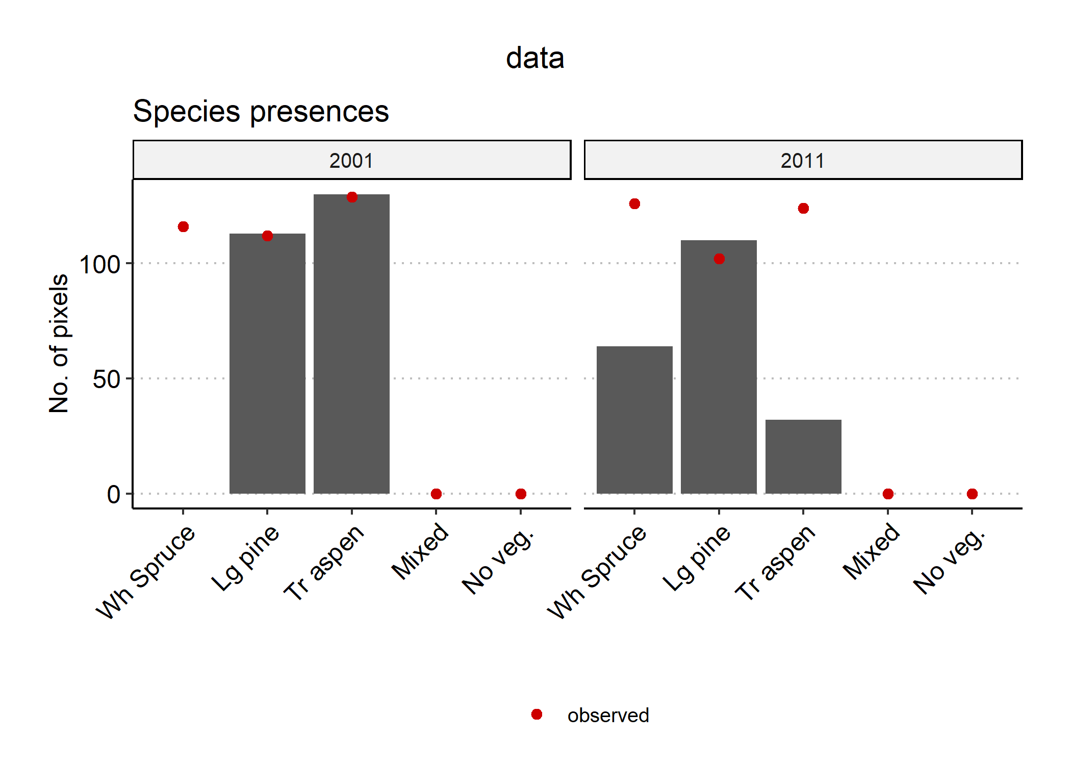
Biomass_validationKNN automatically generates plots showing a visual comparison between simulated and observed species presences (right) across the landscape, and relative species biomass per pixel (left).

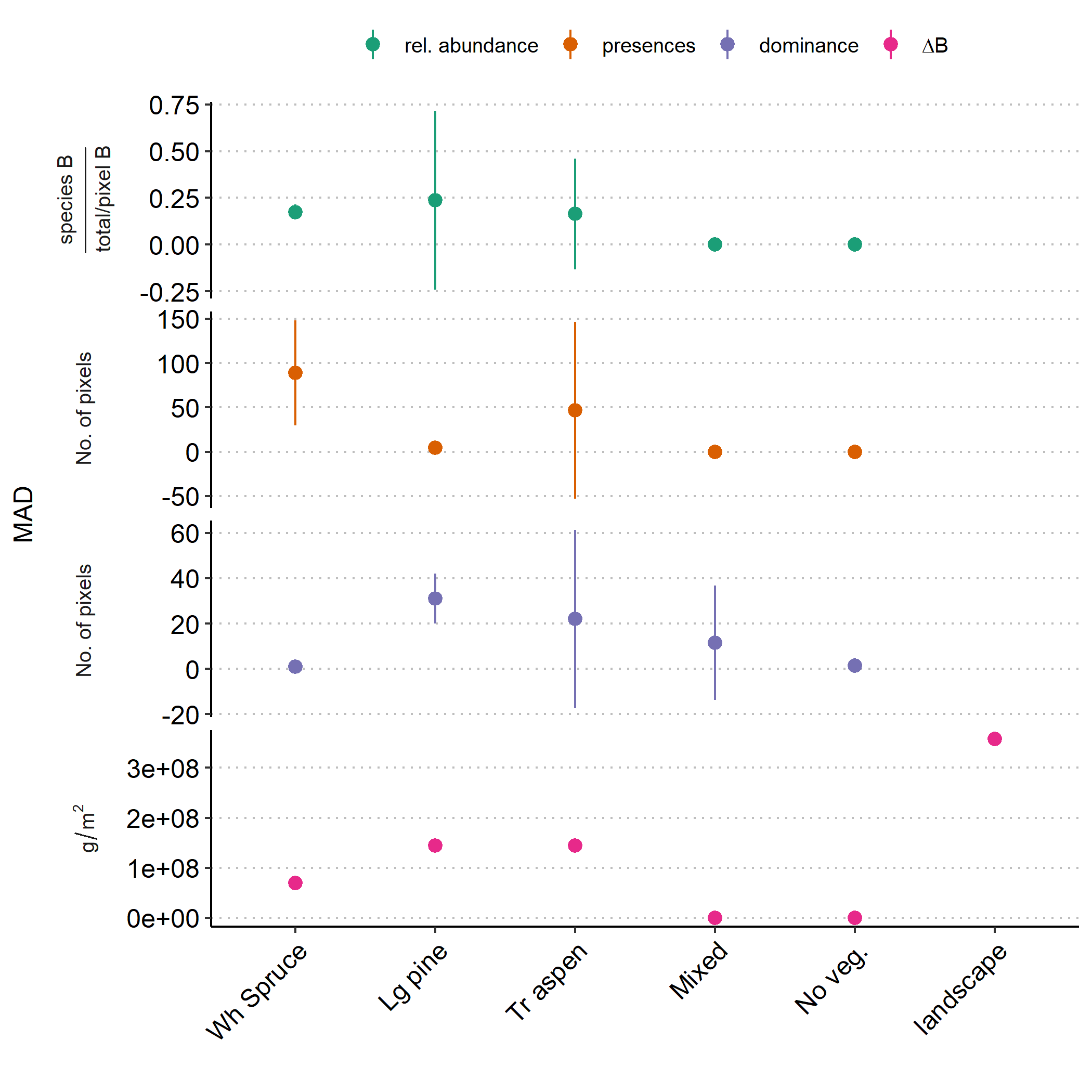
Figure 5.1: Biomass_validationKNN automatically generates plots showing a visual comparison between simulated and observed species presences (right) across the landscape, and relative species biomass per pixel (left).

$A plot of landscape-wide mean absolute deviations (MAD) from (top to bottom) observed mean relative abundance, no. of presences, no. of pixels where the species is dominant and $\Delta$B.$

Figure 5.2: A plot of landscape-wide mean absolute deviations (MAD) from (top to bottom) observed mean relative abundance, no. of presences, no. of pixels where the species is dominant and $\Delta$B.

$Diagnostic plot of observed changes in biomass and age $\Delta$B and $\Delta$Age, respectively).$

Figure 5.3: Diagnostic plot of observed changes in biomass and age $\Delta$B and $\Delta$Age, respectively).

5.4 References

Barros, C., Luo, Y., Chubaty, A.M., Eddy, I.M.S., Micheletti, T., Boisvenue, C., et al. (in review). Empowering ecologists with a PERFICT workflow: Seamlessly linking data, parameterization, prediction, validation and visualization.

Beaudoin, A., Bernier, P.Y., Villemaire, P., Guindon, L. & Guo, X.J. (2017). Species composition, forest properties and land cover types across canada’s forests at 250m resolution for 2001 and 2011.

Burton, P.J. & Cumming, S.G. (1995b). Potential effects of climatic change on some western canadian forests, based on phenological enhancements to a patch model of forest succession. Water, Air and Soil Pollution, 82, 401–414.

Burton, P.J. & Cumming, S.G. (1995a). Potential effects of climatic change on some western canadian forests, based on phenological enhancements to a patch model of forest succession. Water, Air and Soil Pollution, 82, 401–414.

Chubaty, A.M. & McIntire, E.J.B. (2019). SpaDES: Develop and run spatially explicit discrete event simulation models.

Cosco, J. (2011). COMMON ATTRIBUTE SCHEMA (CAS) FOR FOREST INVENTORIES ACROSS CANADA. BOREAL AVIAN MODELLING PROJECT, CANADIAN BEACONs PROJECT.

Hogg, E.H. (Ted), Brandt, J.P. & Michaelian, M. (2008). Impacts of a regional drought on the productivity, dieback, and biomass of western canadian aspen forests. Canadian Journal of Forest Research, 38, 1373–1384.

Lambert, M.C., Ung, C.H. & Raulier, F. (2005). Canadian national tree aboveground biomass equations. Canadian Journal of Forest Research, 35, 1996–2018.

McIntire, E.J.B. & Chubaty, A.M. (2020). Reproducible: A set of tools that enhance reproducibility beyond package management.

McIntire, E.J.B. & Chubaty, A.M. (2021). SpaDES.experiment: Simulation experiments within the SpaDES ecosystem.

Messier, C., Parent, S. & Bergeron, Y. (1998). Effects of overstory and understory vegetation on the understory light environment in mixed boreal forests. Journal of Vegetation Science, 9, 511–520.

NRCan. (2013). National ecological framework for canada - terrestrial ecozones.

Peng, C., Ma, Z., Lei, X., Zhu, Q., Chen, H., Wang, W., et al. (2011). A drought-induced pervasive increase in tree mortality across canada’s boreal forests. Nature Climate Change, 1, 467–471.

Scheller, R.M. & Domingo, J.B. (2011). LANDIS-II model v6.0 user guide.

Scheller, R.M. & Domingo, J.B. (2012). LANDIS-II model v6.0 conceptual description.

Scheller, R.M. & Miranda, B.R. (2015a). LANDIS-II biomass succession v3.2 extension – user guide.

Scheller, R.M. & Miranda, B.R. (2015b). LANDIS-II biomass succession v3.2 extension user guide.

Scheller, R.M. & Mladenoff, D.J. (2004). A forest growth and biomass module for a landscape simulation model, LANDIS: design, validation, and application. Ecological Modelling, 180, 211–229.

Stall, S., Yarmey, L., Cutcher-Gershenfeld, J., Hanson, B., Lehnert, K., Nosek, B., et al. (2019). Make scientific data FAIR. Nature, 570, 27–29.

Sturtevant, B.R., Miranda, B.R., Scheller, R.M. & Shinneman, D. (2018). LANDIS-II dynamic fire system extension v3.0 – user guide.

Ung, C.-H., Bernier, P. & Guo, X.-J. (2008). Canadian national biomass equations: New parameter estimates that include british columbia data. Canadian Journal of Forest Research, 38, 1123–1132.

Wickham, H. (2011). testthat: Get Started with Testing. The R Journal, 3, 5.

Wilkinson, M.D., Dumontier, M., Aalbersberg, Ij.J., Appleton, G., Axton, M., Baak, A., et al. (2016). The FAIR guiding principles for scientific data management and stewardship. Scientific Data, 3, 160018.

Yang, J., He, H.S., Shifley, S.R., Thompson, F.R. & Zhang, Y. (2011). An innovative computer design for modeling forest landscape change in very large spatial extents with fine resolutions. Ecological Modelling, 222, 2623–2630.

Raw data layers downloaded by the module are saved in `dataPath(sim)`, which can be controlled via `options(reproducible.destinationPath = …)`.↩︎

LandR Validation Modules